1. Install the imprinting package
The imprinting package isn’t yet available on CRAN, so it can’t yet be
installed using the normal install.packages("imprinting")
command in R. (But this feature is coming soon!)
For now, we have to install the package from github using the following steps.
1.1 Install the devtools package
If prompted: you do not need to researt R prior to lading, and you do not need to install from souce.
install.packages("devtools", repos='http://cran.us.r-project.org')1.2 Load the devtools package
Now that we have devtools installed, we can use the
install_github() function to install the imprinting
package.
1.3 Install the imprinting package from github
This builds and installs the package using source files from https://github.com/cobeylab/imprinting.
devtools::install_github("cobeylab/imprinting") 2. Use the package to calculate imprinting probabilities
The main reason to use the imprinting package is to
calculate birth year-specific probabilities of imprinting to a specific
subtype of influenza A. You can read more about the biology and methods
behind these calculations in Gostic et
al. (2016).
2.1 Calculate imprinting probabilities for one country and year of observation
Use the function get_imprinting_probabilities(). Run
?get_imprinting_probabilities for help.
get_imprinting_probabilities(observation_years = 2022, countries = "United States")
#> # A tibble: 420 × 5
#>     year country       birth_year subtype imprinting_prob
#>    <dbl> <chr>              <dbl> <chr>             <dbl>
#>  1  2022 United States       2022 A/H1N1        0.0000297
#>  2  2022 United States       2021 A/H1N1        0.0000679
#>  3  2022 United States       2020 A/H1N1        0.0702
#>  4  2022 United States       2019 A/H1N1        0.152
#>  5  2022 United States       2018 A/H1N1        0.171
#>  6  2022 United States       2017 A/H1N1        0.147
#>  7  2022 United States       2016 A/H1N1        0.225
#>  8  2022 United States       2015 A/H1N1        0.169
#>  9  2022 United States       2014 A/H1N1        0.308
#> 10  2022 United States       2013 A/H1N1        0.321
#> # … with 410 more rows
The function returns a tibble wtih five columns:
subtype, year, country,
birth_year, and imprinting_prob. The column
imprinting_prob gives the probability that someone born in
birth_year and observed in year has imprinted
to subtype.
We can run the same command use the df_format='wide'
option to output the same results in wide format. This displays all
imprinting probabilities for the cohort side-by-side
get_imprinting_probabilities(observation_years = 2022,
                             countries = "United States",
                             df_format = 'wide')
#> # A tibble: 105 × 7
#>     year country       birth_year `A/H1N1` `A/H2N2` `A/H3N2` naive
#>    <dbl> <chr>              <dbl>    <dbl>    <dbl>    <dbl> <dbl>
#>  1  2022 United States       1918        1        0        0     0
#>  2  2022 United States       1919        1        0        0     0
#>  3  2022 United States       1920        1        0        0     0
#>  4  2022 United States       1921        1        0        0     0
#>  5  2022 United States       1922        1        0        0     0
#>  6  2022 United States       1923        1        0        0     0
#>  7  2022 United States       1924        1        0        0     0
#>  8  2022 United States       1925        1        0        0     0
#>  9  2022 United States       1926        1        0        0     0
#> 10  2022 United States       1927        1        0        0     0
#> # … with 95 more rows
2.2 Why do we specify the observation_year?
The observation_year affects imprinting probabilities in
birth cohorts who are young enough to still be in the process of
imprinting. Our model assumes that everyone has been infected by
influenza before age 12, so in cohorts <12 years of age at the time
of observation, imprinting probabilities depend on the observation
year.
E.g. consider the cohort born in 2000:
- If the observation year is 2005, then this birth cohort is five years old, and still young enough to remain naive to influenza. The outputs below show that 22.9% of the cohort has not yet imprinted to any subtype.
- If we calculate imprinting probabilities for the same birth cohort observed in 2011 (at age 11), the model shows that most of the cohort has imprinted, but there is still a very small non-zero probability of remaining naive.
- When the cohort reaches age 12, (observation year 2012) the model enforces the assumption that everyone in the cohort has imprinted. It normalizes the probabilities of subtype-specific imprinting so that the H1N1, H2N2, and H3N2-specific probabilities sum to 1, and it sets the naive probability to zero.
- Once the cohort reaches age 12, imprinting probabilities are fixed. The outputs below show that imprinting probabilities for the 2000 cohort are identical if observed at age 12 (in 2012), or at age 22 (in 2022).
Note: we added the age_at_observation column to the outputs below for clarity.
get_imprinting_probabilities(observation_years = c(2005, 2011, 2012, 2022),
                             countries = "United States",
                             df_format = 'wide') %>%
  dplyr::filter(birth_year == 2000) %>%
  mutate(age_at_observation = year-birth_year) %>%
  select(c(1,2,3,8,4:7))
#> # A tibble: 4 × 8
#>    year country    birth_year age_at_observat… `A/H1N1` `A/H2N2` `A/H3N2`  naive
#>   <dbl> <chr>           <dbl>            <dbl>    <dbl>    <dbl>    <dbl>  <dbl>
#> 1  2005 United St…       2000                5    0.196        0    0.574 0.229
#> 2  2011 United St…       2000               11    0.322        0    0.667 0.0104
#> 3  2012 United St…       2000               12    0.324        0    0.676 0
#> 4  2022 United St…       2000               22    0.324        0    0.676 0
2.2 View a list of the available countries
We can only calculate imprinting probabilities for countries with data in WHO Flu Net. The input name and spelling must match the outputs below:
show_available_countries() %>%
  print(n = 200)
#> # A tibble: 175 × 1
#>     country
#>     <chr>
#>   1 Afghanistan
#>   2 Albania
#>   3 Algeria
#>   4 Angola
#>   5 Anguilla
#>   6 Antigua and Barbuda
#>   7 Argentina
#>   8 Armenia
#>   9 Aruba
#>  10 Australia
#>  11 Austria
#>  12 Azerbaijan
#>  13 Bahamas
#>  14 Bahrain
#>  15 Bangladesh
#>  16 Barbados
#>  17 Belarus
#>  18 Belgium
#>  19 Belize
#>  20 Bermuda
#>  21 Bhutan
#>  22 Bolivia
#>  23 Bosnia and Herzegovina
#>  24 Brazil
#>  25 British Virgin Islands
#>  26 Bulgaria
#>  27 Burkina Faso
#>  28 Cabo Verde
#>  29 Cambodia
#>  30 Cameroon
#>  31 Canada
#>  32 Cayman Islands
#>  33 Central African Republic
#>  34 Chad
#>  35 Chile
#>  36 China
#>  37 Colombia
#>  38 Congo
#>  39 Costa Rica
#>  40 Cote d'Ivoire
#>  41 Croatia
#>  42 Cuba
#>  43 Cyprus
#>  44 Czechia
#>  45 Democratic Republic of Congo
#>  46 Denmark
#>  47 Dominica
#>  48 Dominican Republic
#>  49 Ecuador
#>  50 Egypt
#>  51 El Salvador
#>  52 Estonia
#>  53 Ethiopia
#>  54 Fiji
#>  55 Finland
#>  56 France
#>  57 French Guiana
#>  58 Gambia
#>  59 Georgia
#>  60 Germany
#>  61 Ghana
#>  62 Greece
#>  63 Grenada
#>  64 Guadeloupe
#>  65 Guatemala
#>  66 Guinea
#>  67 Guinea-Bissau
#>  68 Guyana
#>  69 Haiti
#>  70 Honduras
#>  71 Hungary
#>  72 Iceland
#>  73 India
#>  74 Indonesia
#>  75 Iran
#>  76 Iraq
#>  77 Ireland
#>  78 Israel
#>  79 Italy
#>  80 Jamaica
#>  81 Japan
#>  82 Jordan
#>  83 Kazakhstan
#>  84 Kenya
#>  85 Kosovo
#>  86 Kuwait
#>  87 Kyrgyzstan
#>  88 Laos
#>  89 Latvia
#>  90 Lebanon
#>  91 Lithuania
#>  92 Luxembourg
#>  93 Madagascar
#>  94 Malaysia
#>  95 Maldives
#>  96 Mali
#>  97 Malta
#>  98 Martinique
#>  99 Mauritania
#> 100 Mauritius
#> 101 Mexico
#> 102 Moldova
#> 103 Mongolia
#> 104 Montenegro
#> 105 Morocco
#> 106 Mozambique
#> 107 Myanmar
#> 108 Namibia
#> 109 Nepal
#> 110 Netherlands
#> 111 New Caledonia
#> 112 New Zealand
#> 113 Nicaragua
#> 114 Niger
#> 115 Nigeria
#> 116 North Korea
#> 117 North Macedonia
#> 118 Norway
#> 119 Oman
#> 120 Pakistan
#> 121 Palestine
#> 122 Panama
#> 123 Papua New Guinea
#> 124 Paraguay
#> 125 Peru
#> 126 Philippines
#> 127 Poland
#> 128 Portugal
#> 129 Qatar
#> 130 Romania
#> 131 Russia
#> 132 Rwanda
#> 133 Saint Kitts and Nevis
#> 134 Saint Lucia
#> 135 Saint Vincent and the Grenadines
#> 136 Saudi Arabia
#> 137 Senegal
#> 138 Serbia
#> 139 Seychelles
#> 140 Sierra Leone
#> 141 Singapore
#> 142 Slovakia
#> 143 Slovenia
#> 144 South Africa
#> 145 South Korea
#> 146 South Sudan
#> 147 Spain
#> 148 Sri Lanka
#> 149 Sudan
#> 150 Suriname
#> 151 Sweden
#> 152 Switzerland
#> 153 Syria
#> 154 Tajikistan
#> 155 Tanzania
#> 156 Thailand
#> 157 Timor
#> 158 Togo
#> 159 Trinidad and Tobago
#> 160 Tunisia
#> 161 Turkey
#> 162 Turkmenistan
#> 163 Turks and Caicos
#> 164 Uganda
#> 165 Ukraine
#> 166 United Arab Emirates
#> 167 United Kingdom
#> 168 United States
#> 169 Uruguay
#> 170 Uzbekistan
#> 171 Venezuela
#> 172 Vietnam
#> 173 Yemen
#> 174 Zambia
#> 175 Zimbabwe
2.3 Generate probabilities for many countries and observation years
many_probabilities = get_imprinting_probabilities(observation_years = c(2000, 2019, 2022),
                                                  countries = c('Brazil', 'Afghanistan', 'Estonia', 'Finland'))
## Store the outputs in a variable called many_probabilities
many_probabilities ## View the outputs in the console
#> # A tibble: 5,040 × 5
#>     year country     birth_year subtype imprinting_prob
#>    <dbl> <chr>            <dbl> <chr>             <dbl>
#>  1  2000 Brazil            2022 A/H1N1          0.331
#>  2  2019 Brazil            2022 A/H1N1          0.197
#>  3  2022 Brazil            2022 A/H1N1          0
#>  4  2000 Afghanistan       2022 A/H1N1          0.536
#>  5  2019 Afghanistan       2022 A/H1N1          0.110
#>  6  2022 Afghanistan       2022 A/H1N1          0.00138
#>  7  2000 Estonia           2022 A/H1N1          0.485
#>  8  2019 Estonia           2022 A/H1N1          0.188
#>  9  2022 Estonia           2022 A/H1N1          0
#> 10  2000 Finland           2022 A/H1N1          0.239
#> # … with 5,030 more rows
Alternatively, you can view the outputs in a separate window or save them as a .csv file on your hard drive.
# View the outputs in a separate window.
View(many_probabilities)

# Save the outputs as a .csv file in your current working directory.
write_csv(many_probabilities, 'many_probabilities.csv')
3. Plot the outputs
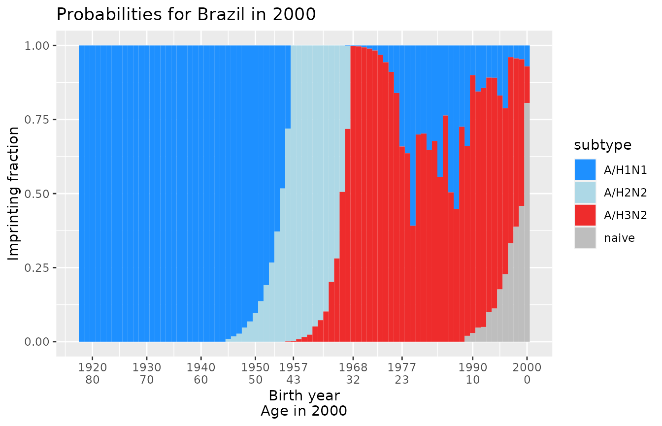
3.1 Plot the first country-year combination in the output data frame
plot_one_country_year() takes a long-formatted output
data frame and plots the first country and year combination.
head(many_probabilities)
#> # A tibble: 6 × 5
#>    year country     birth_year subtype imprinting_prob
#>   <dbl> <chr>            <dbl> <chr>             <dbl>
#> 1  2000 Brazil            2022 A/H1N1          0.331
#> 2  2019 Brazil            2022 A/H1N1          0.197
#> 3  2022 Brazil            2022 A/H1N1          0
#> 4  2000 Afghanistan       2022 A/H1N1          0.536
#> 5  2019 Afghanistan       2022 A/H1N1          0.110
#> 6  2022 Afghanistan       2022 A/H1N1          0.00138
plot_one_country_year(many_probabilities) 
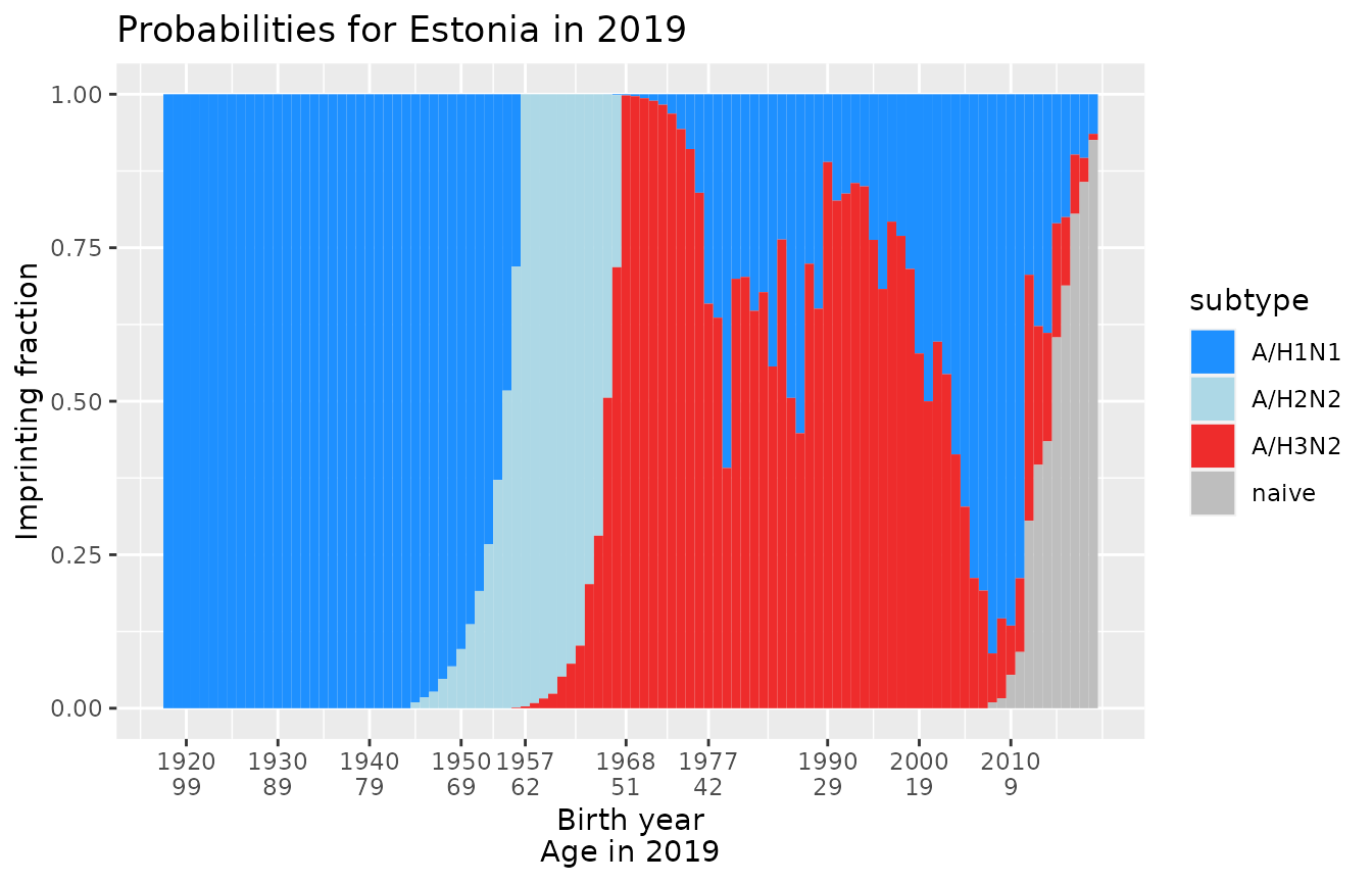
Select a specific country and year to plot
You can use filter() to select a specific country and
year for plotting.
plot_one_country_year(many_probabilities %>%
                        dplyr::filter(country == 'Estonia', year == 2019))
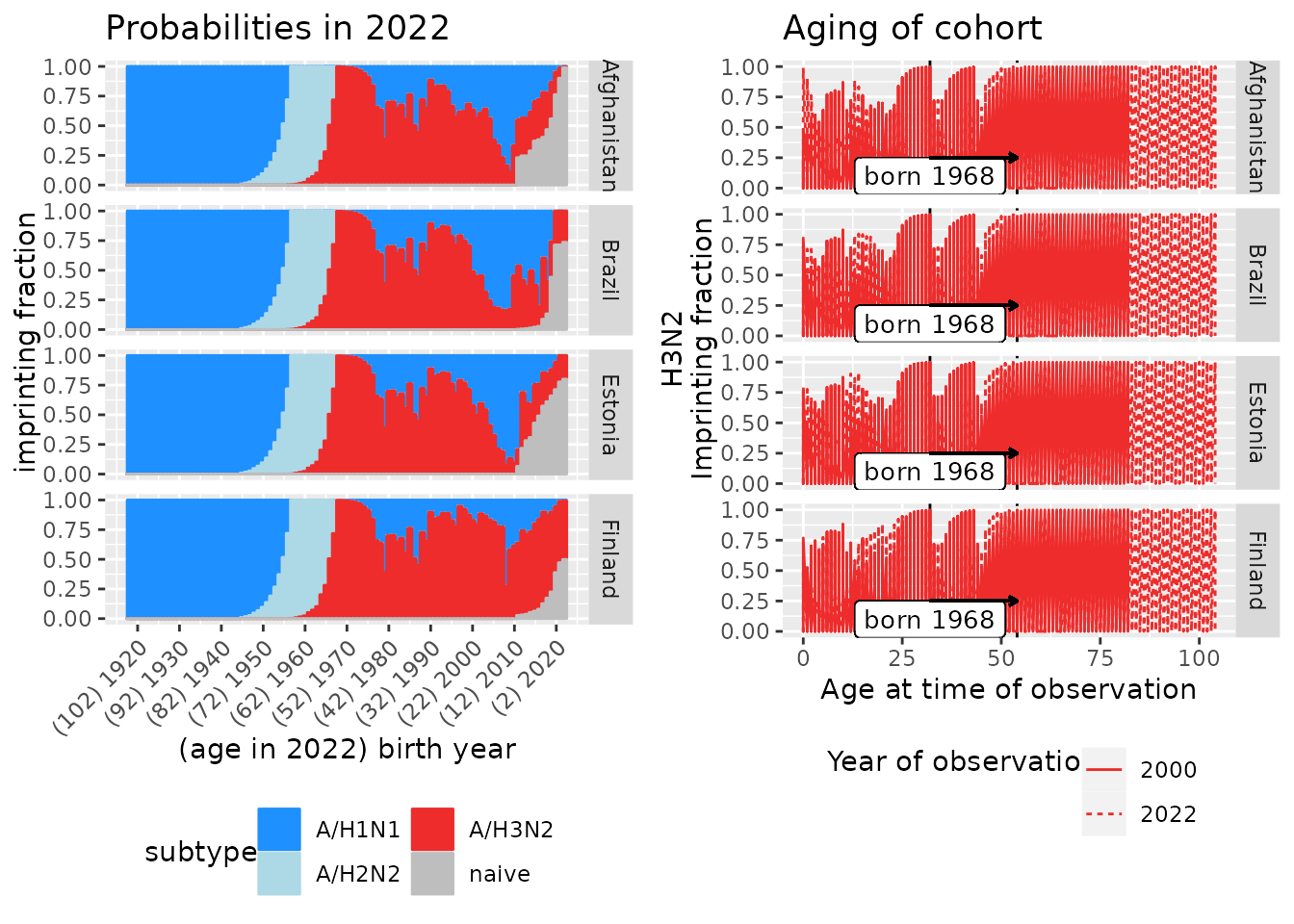
3.2 Plot up to five countires at a time
plot_many_country_years() generates a plot of the first
five countries in the imprinting outputs, across an arbitrary number of
years.
- The plots on the left show imprinting probabilities for the latest observation year
- The plots on the right show how H3N2 imprinting probabilities have changed as cohorts grow older from the earliest to the latest observation year in the outputs. The vertical lines and arrow show aging of the 1968 birth cohort.
plot_many_country_years(many_probabilities)
4. Explore the underlying data and components of the imprinting probabilities
Get the fraction of influenza circulation caused by each subtype in
each epidemic year from 1918-2022 in the United States using
get_country_cocirculation. Run
?get_country_cocirculation_data for notes on data
sources.
get_country_cocirculation_data('United States', 2022)
#> # A tibble: 105 × 9
#>     year `A/H1N1` `A/H2N2` `A/H3N2`     A B     group1 group2 data_from
#>    <dbl>    <dbl>    <dbl>    <dbl> <dbl> <lgl>  <dbl>  <dbl> <chr>
#>  1  1918        1        0        0     1 NA         1      0 Historical_assump…
#>  2  1919        1        0        0     1 NA         1      0 Historical_assump…
#>  3  1920        1        0        0     1 NA         1      0 Historical_assump…
#>  4  1921        1        0        0     1 NA         1      0 Historical_assump…
#>  5  1922        1        0        0     1 NA         1      0 Historical_assump…
#>  6  1923        1        0        0     1 NA         1      0 Historical_assump…
#>  7  1924        1        0        0     1 NA         1      0 Historical_assump…
#>  8  1925        1        0        0     1 NA         1      0 Historical_assump…
#>  9  1926        1        0        0     1 NA         1      0 Historical_assump…
#> 10  1927        1        0        0     1 NA         1      0 Historical_assump…
#> # … with 95 more rows
Get the circulation intensity of influenza A in each epidemic year
using get_country_intensity_data().
- Intensity of 1 is average. Higher values indicate more influenza A circulation, lower values indicate less circulation.
See ?get_country_intensity_data for details on
underlying data.
get_country_intensity_data(country = 'China', max_year = 2022)
#> # A tibble: 113 × 2
#>     year intensity
#>    <dbl>     <dbl>
#>  1  1911      1
#>  2  1912      1
#>  3  1913      1
#>  4  1914      1
#>  5  1915      1.12
#>  6  1916      1.29
#>  7  1917      1.23
#>  8  1918      2.5
#>  9  1919      2.5
#> 10  1920      1.87
#> # … with 103 more rows
Get the probability that an individual imprinted 0, 1, 2, … 12 years after birth
Use the function get_p_infection_year()
probs = get_p_infection_year(birth_year = 2000,
                     observation_year = 2022,
                     intensity_df = get_country_intensity_data('Mexico', 2022),
                     max_year = 2022)
names(probs) = as.character(2000+(0:12))
probs
#>        2000        2001        2002        2003        2004        2005
#> 0.014797424 0.038348694 0.014337222 0.078764203 0.015525076 0.093914147
#>        2006        2007        2008        2009        2010        2011
#> 0.007673805 0.058215925 0.017624843 0.462559063 0.119102374 0.013750798
#>        2012
#> 0.036377222
sum(probs) ## Raw probabilities are not yet normalized.
#> [1] 0.9709908

norm_probs = probs/sum(probs) ## Normalize
sum(norm_probs)
#> [1] 1